|
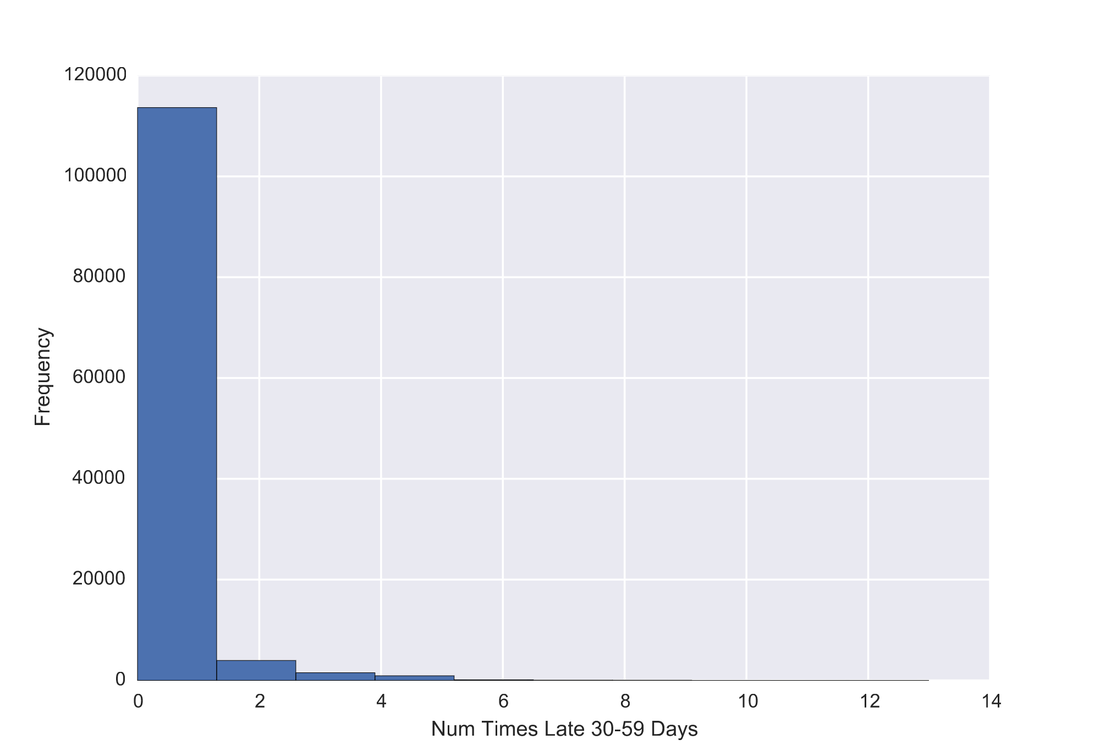
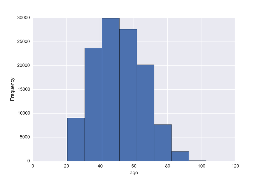
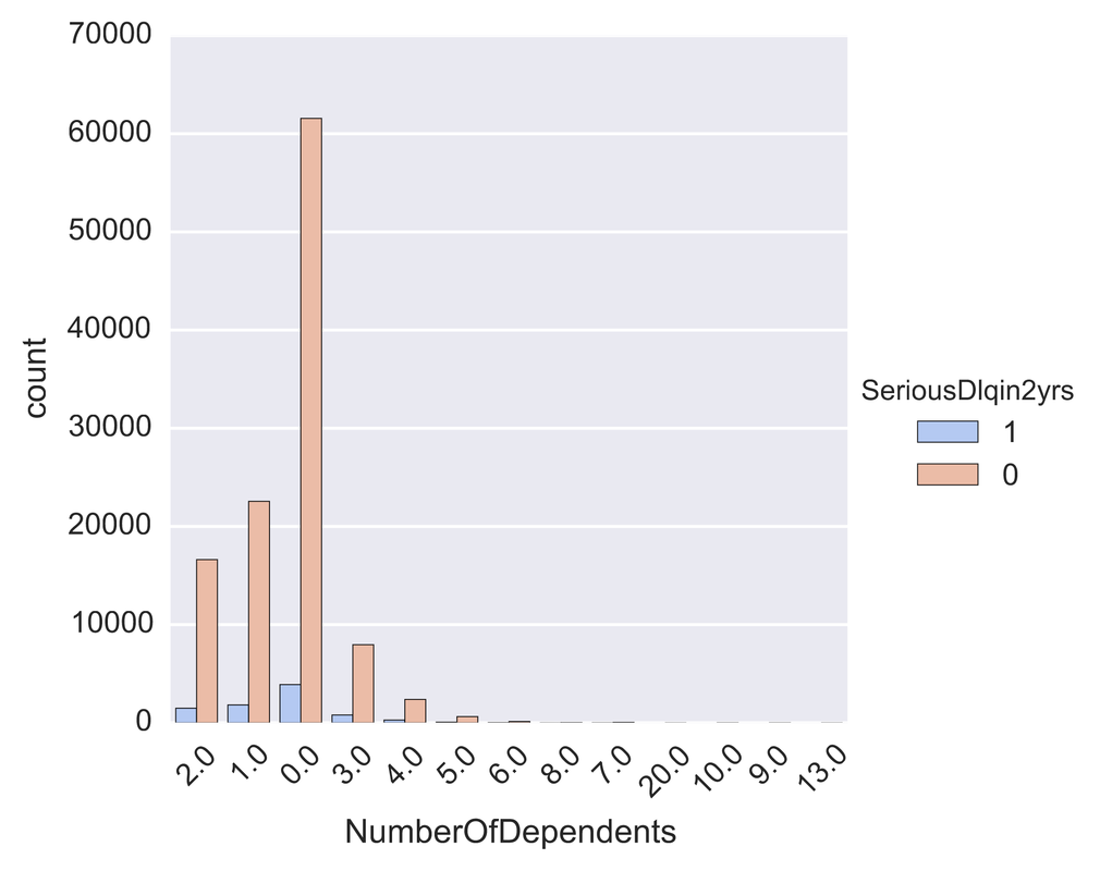
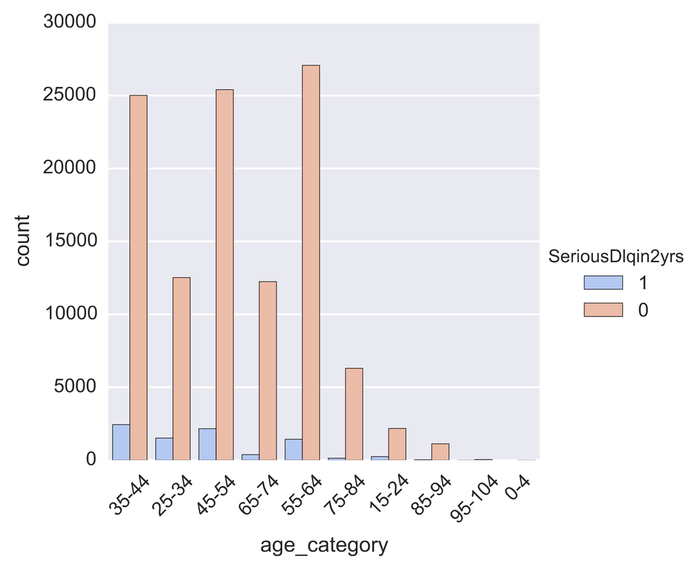
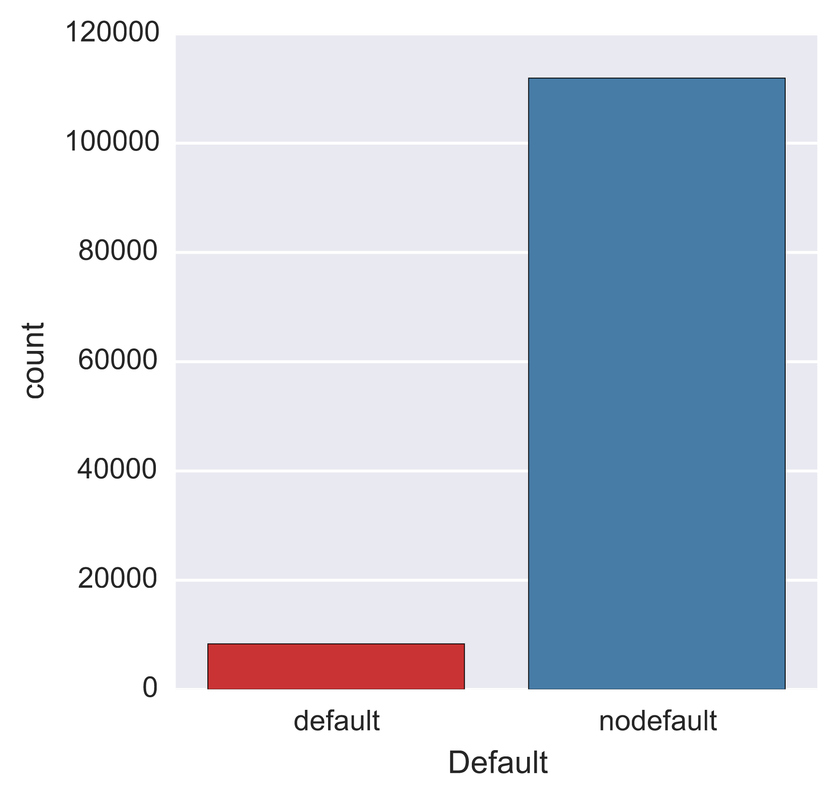
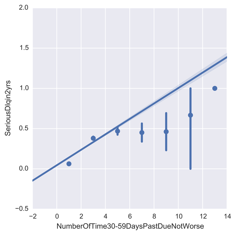
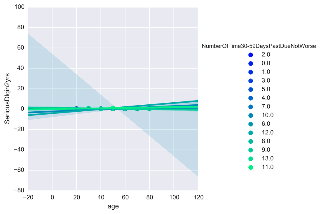
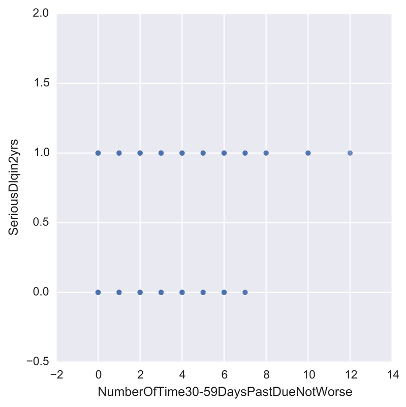
One problem banks are interested in is determining the credit score of their customers in order to predict the likelihood that their customers would default on a potential loan. In this blog post I will talk about the project I worked on that dealt with this problem. I obtained data from: https://www.kaggle.com/c/GiveMeSomeCredit I used Python to work on this data set. I started with Logistic Regression to carry out my analyses. Because the training set had lots of NA values, I first got rid of the entries that contained any NA values The "30-59DaysPastDueNotWorse" variable contained values 96 and 98, which are typos, so I replaced them with the median of 30-59DaysPastDueNotWorse I then generated histograms of the 'age' and 'NumberOfTime30-59DaysPastDueNotWorse' variables I then generated a KDE plot to further visualize the data. The KDE plot is similar to a histogram in that it treats each data point as a Gaussian distribution and then takes the cumulative probability function 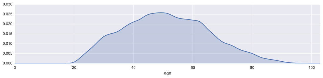 I also wanted to generate plots that show how many of the entries contained defaults and non-defaults, along with factor plots (using the Seaborn package) that shows how the defaults varies depending on the age and number of dependents of each person I then generated linear plots using Seaborn to see how the number of defaults correlates with the 'NumberOfTime30-59DaysPastDueNotWorse' variable I then proceeded with Logistic Regression. I first set the dependent variable as the defaults and converted it into a 1-d array as required by Scikit-learn I then computed the score by using Logistic Regression on the entire training set. I obtained a score of 93.06%. However, this was only a marginal improvement from the actual percentage of non-defaults in the dataset, which is 93.05% To improve on this score, I then tried Regularization with the Lasso l1 penalty. I then split the training set into a training and validation/test set. Python automatically converts 75% of the original set into a new training set and the remaining 25% becomes the validation set. The plot below shows the coefficients as a function of the log of C (where C=1/lambda, where lambda is the penalty term. The greater the lambda, the more the coefficients of the predictors tends towards 0, thus eliminating the irrelevant predictors) 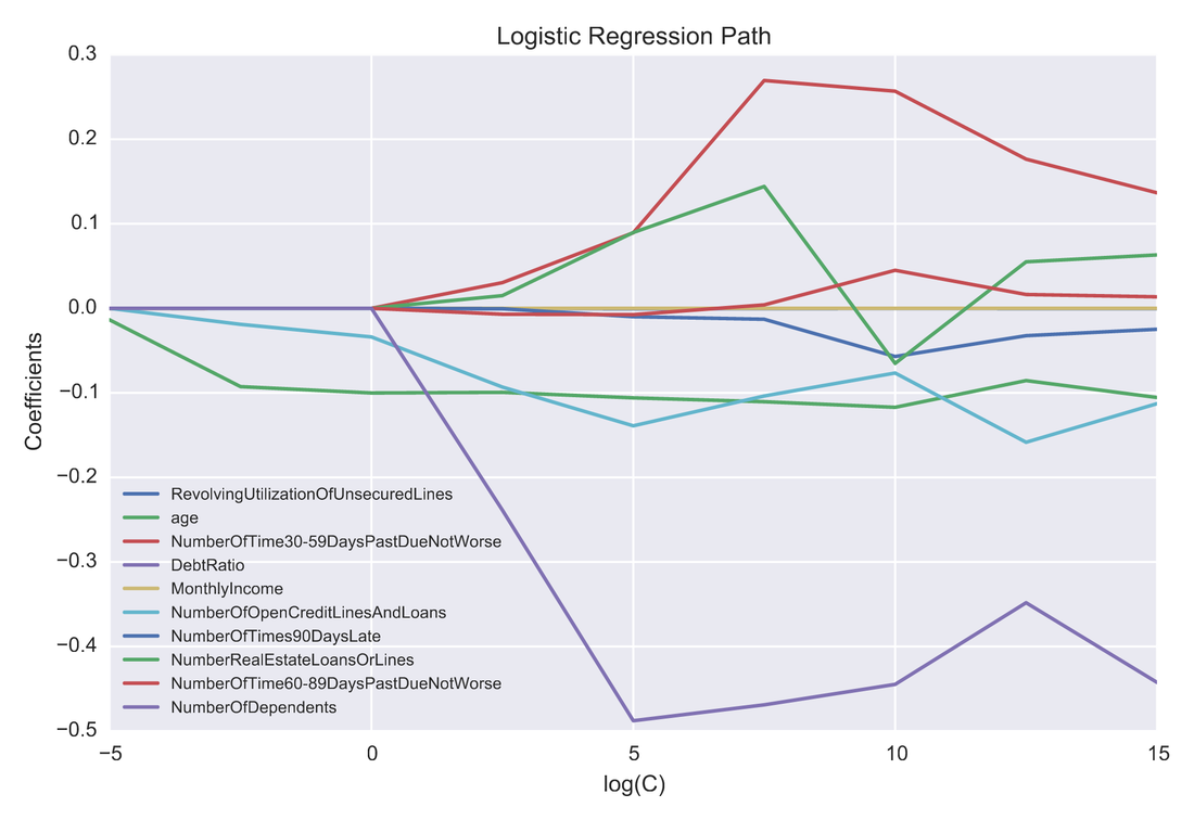 Many of the coefficients go towards 0 when C=0 (or lambda = inf). The accuracy scores I obtained were 1.0 for C values = 1, 316.2, 100000, 3.16e7, etc. However, the score was .9301 when C=1e-5 and .99963 when C=.003 (logC = -2.5). From the plot, it is hard to determine which predictors become 0 due to increasing C. I concluded that the most relevant predictors were DebtRatio, age, NumberRealEstateLoansOrLines, and NumberOfOpenCreditLinesAndLoans.
I then used only these relevant predictors in another Logistic Regression analysis. However, with just these predictors, the accuracy dropped to .9277 For future studies, I plan to utilize Random Forest and Support Vector Machine to compare the accuracy score with Logistic Regression. I also want to see if using an ensemble of these methods can further improve the accuracy score Full details of the code at: https://github.com/jk34/Kaggle_Credit_Default_Loan
0 Comments
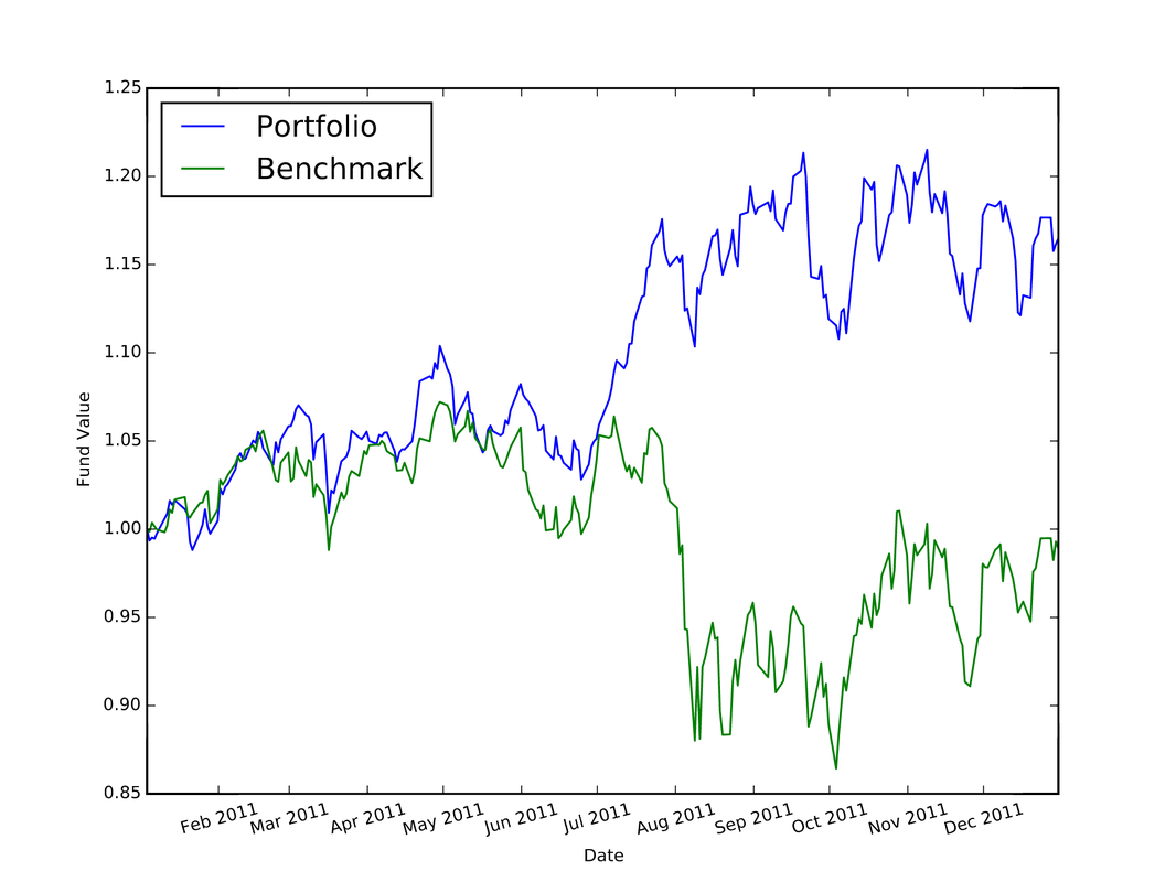 I used Python to complete the assignments for the coursera course "Computational Investing". The description of the course and the assignments is located at: http://wiki.quantsoftware.org/index.php?title=Computational_Investing_I For the assignments, I used the QSTK package, which supports portfolio construction and management. It is described further at: http://wiki.quantsoftware.org/index.php?title=QuantSoftware_ToolKit For the 1st assignment, I wrote the program hw1.py. which simulates how the stocks in a given portfolio perform over time and computes the statistics of the final values of the stocks to see how much profit/loss you got with this portfolio. The program also contains a portfolio optimizer to test every "legal" set of allocations to the 4 given stocks to see which allocation of stocks produces the best portfolio. The plot below (and which is also located in my Github repository at https://github.com/jk34/Computational_Investing_Python_Coursera) shows the value of the portfolio compared to a benchmark (S&P 500 index) over time For the 2nd assignment, the program hw2.py (code details at my github page) conducts "event studies" to see how stock price "events" affect future prices. An event is defined as when the actual close of a stock price drops below $5.00 when its actual close was at least $5 the previous day. It uses the Event Profiler provided in QSTK. The event profiler output, which allows us to see how stocks perform after a market event, is displayed in the plot below 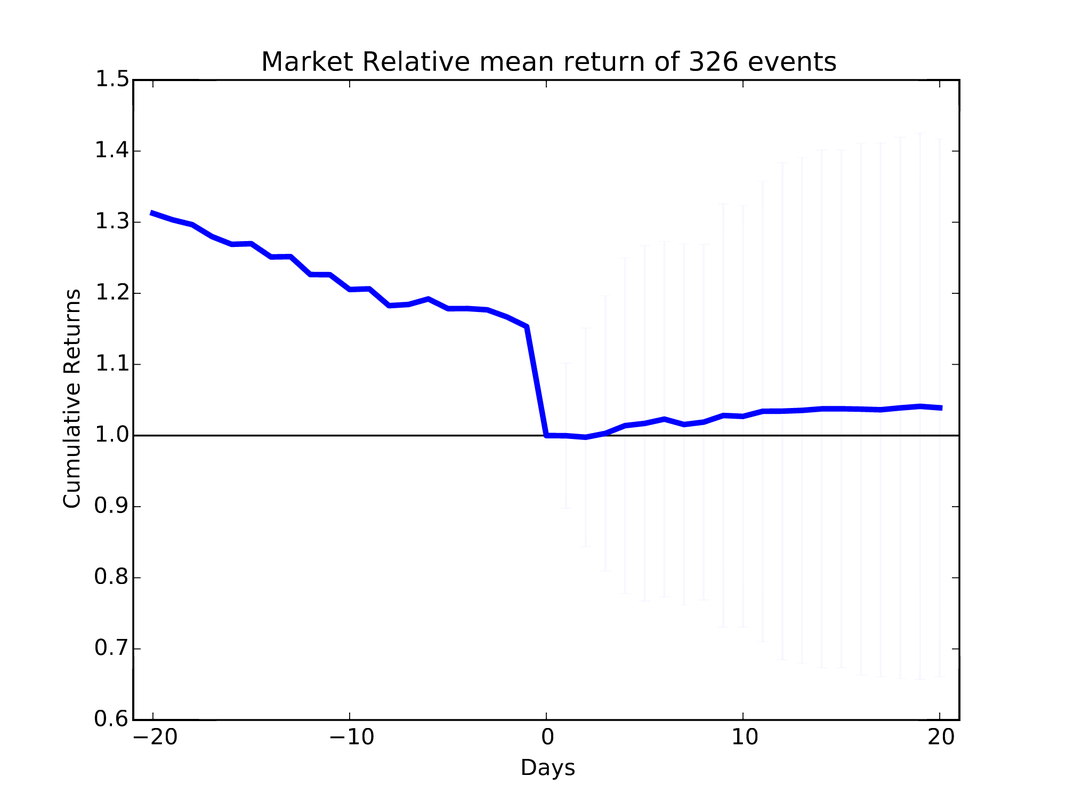 For the 3rd assignment, I first wrote "hw3_marketsim.py", which creates a market simulator that accepts trading orders (buy and/or sell stocks) and keeps track of the value of the portfolio containing all the equities by using the values of the stocks in historical data. The market simulator is used if you have a trading strategy containing trades you want to execute. The simulator then simulates those trades by executing them "hw3_analyze.py" then analyzes the performance of that portfolio by computing the Sharpe Ratio, Standard Deviation, Average Daily Return of Fund, and Total/Cumulative Return of your strategy in order to measure the performance of that strategy. The "marketsim-guidelines.pdf" file explains how to build the simulator, and is located at http://wiki.quantsoftware.org/index.php?title=CompInvesti_Homework_3 The plot below shows the value of the portfolio compared to a benchmark (S&P 500 index) over time 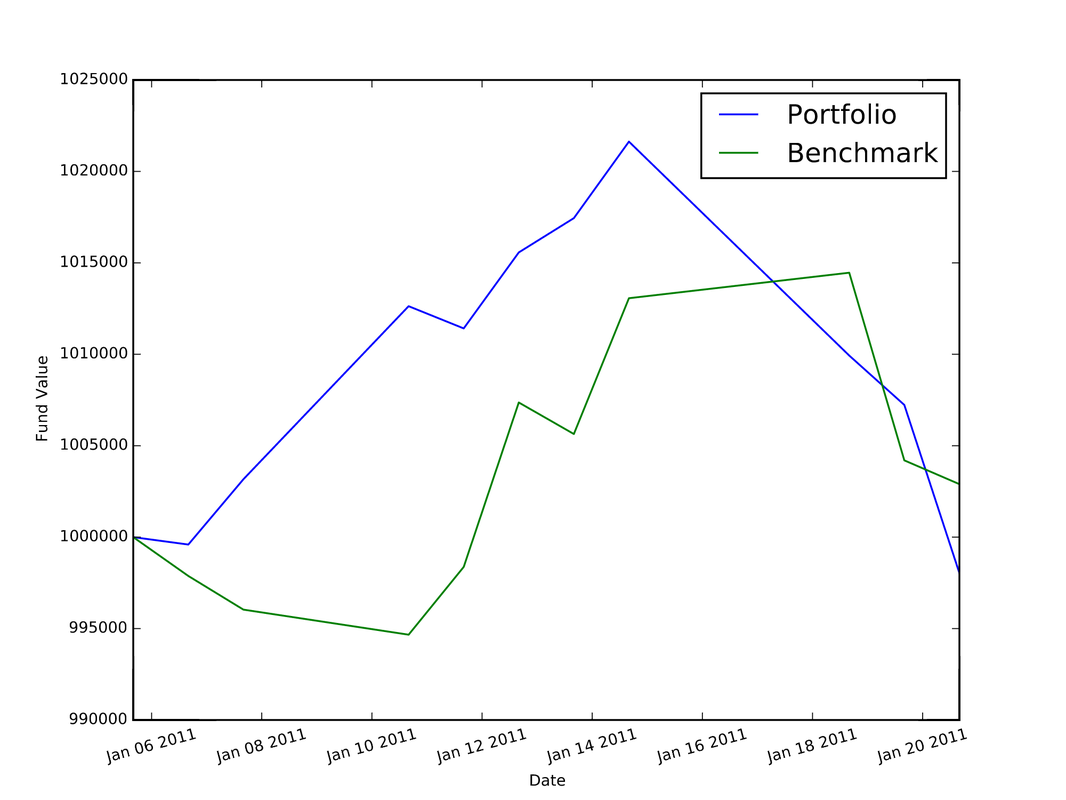 For the 4th assignment, my program "hw4.py" combines the Event Study in "hw2.py" with the market simulator in "hw3_marketsim.py" by taking the output of the Event Study in hw2.py as a trading strategy and then inputting it into the market simulator I created in "hw3.py". This program creates a trading strategy by specifying that when an event occurs, we will buy 100 shares of the equity on that day and then sell it 5 trading days later. The plot below shows the value of the portfolio compared to a benchmark (S&P 500 index) over time 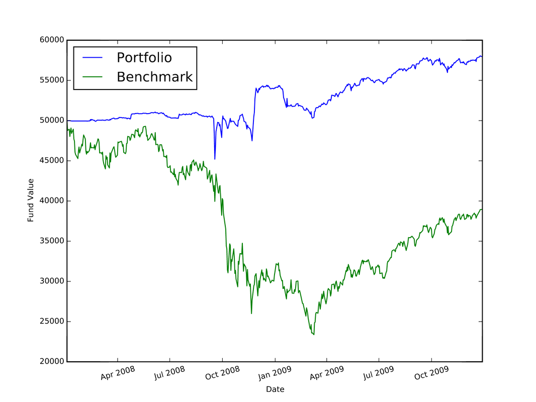 For the 5th assignment, "hw5.py" first computes the rolling mean, the stock price, and upper and lower bands. Then, it computes the Bollinger bands. The results are plotted below 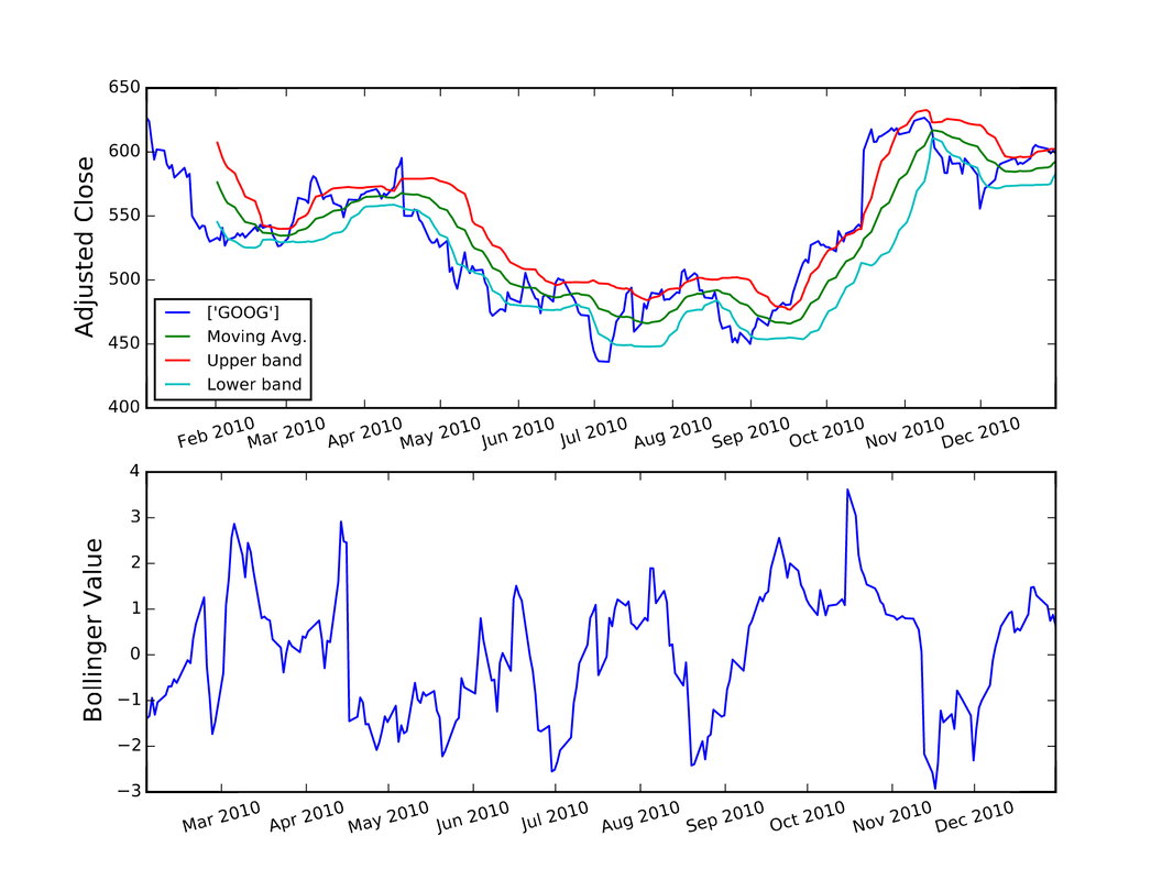 In this blog post I will discuss my work on the data provided for the San Francisco Crime Classification competition by Kaggle. The data and description of the competition is located at: https://www.kaggle.com/c/sf-crime
I ran Linear Discriminant Analysis and Random Forest on the training data in order to predict the type of crime that occurred in the test set. I could not try Principal Component Analysis to perform dimension reduction because the data only contains categorical variables. As explained in the book "Introduction to Statistical Learning" by Tibshirani et al., because the outcome variable in the dataset has more than 2 outcomes, it is better to use LDA than logistic regression because the parameter estimates are unstable for logistic regression. However, that's not true for LDA I got a better value for the log-loss score when using LDA than with Random Forest. For LDA, I used the first 100000 rows of the validation set and the remaining rows as the training set for Cross Validation. The log-loss I obtained was 2.547. I could not do this with Random Forest because I kept getting errors with memory size because Random Forest uses up alot of the computer's RAM. Therefore, I had to use smaller data for the training and validation set. The log-loss was -3.18 when I used only the rows 850001:878049 of the original training set file as the training set and the 1st 100 rows of that as the validation set and using ntree=100. I then tried to get a better log-loss, so I then got 6 samples that contained each outcome for the dependent variable (crime Category) using dplyr as the training set. I then used the first 50000 of the training set file as the validation set for Cross Validation. I then ran Random Forest with 5000 trees and computed the log-loss as 3.856. It worsened to 4.856 when using 200 samples that contained each possible outcome for the crime category. So the log-loss for LDA was better than any of the log-loss values computed from Random Forest I then used k-fold cross validation on LDA before creating a submission file containing the predicted probabilities on the test data provided by Kaggle. With 10 folds, the average log-loss was 2.668. In the future, I plan to modify this by further tuning the parameters for the Random Forest method to get the best possible log-loss You can find the code I used for this analysis at: https://github.com/jk34/Kaggle_SF_Crime_Classification/blob/master/run.r |
AuthorHello world, my name is Jerry Kim. I have a Master's Degree in Physics and years of work experience in Image Processing, Machine Learning, and Deep Learning. I mostly have used C++, Matlab, and Python. I created this website to showcase a small sample of the things that I have worked on Archives
March 2017
Categories |
 RSS Feed
